Pipelines End-to-end on GCP
This guide walks you through a Kubeflow Pipelines sample that runs an MNIST machine learning (ML) model on Google Cloud Platform (GCP).
Introductions
Kubeflow Pipelines is a platform for building and deploying portable, scalable ML workflows based on Docker containers. When you install Kubeflow, you get Kubeflow Pipelines too.
By working through this tutorial, you learn how to deploy Kubeflow on Kubernetes Engine (GKE) and run a pipeline supplied as a Python script. The pipeline trains an MNIST model for image classification and serves the model for online inference (also known as online prediction).
Overview of GCP and GKE
Google Cloud Platform (GCP) is a suite of cloud computing services running on Google infrastructure. The services include compute power, data storage, data analytics, and machine learning.
The Cloud Shell is a browser interface that provides command-line access to cloud resources that you can use to interact with GCP, including the gcloud command and others.
Kubernetes Engine (GKE) is a managed service on GCP where you can deploy containerized applications. You describe the resources that your application needs, and GKE provisions and manages the underlying cloud resources automatically.
Here’s a list of the primary GCP services that you use when following this guide:
The model and the data
This tutorial trains a TensorFlow model on the MNIST dataset, which is a hello world scenario for machine learning.
The MNIST dataset contains a large number of images of hand-written digits in the range 0 to 9, as well as the labels identifying the digit in each image.
After training, the model can classify incoming images into 10 categories
(0 to 9) based on what it’s learned about handwritten images. In other words,
you send an image to the model, and the model does its best to identify the
digit shown in the image.
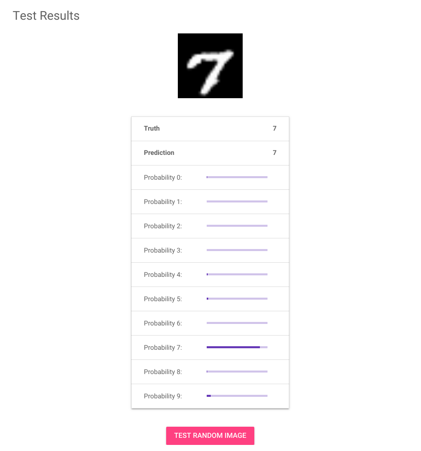
In the above screenshot, the image shows a hand-written 7. This image was the input to the model. The table below the image shows a bar graph for each classification label from 0 to 9, as output by the model. Each bar represents the probability that the image matches the respective label. Judging by this screenshot, the model seems pretty confident that this image is a 7.
Set up your environment
Let’s get started!
Set up your GCP account and SDK
Follow these steps to set up your GCP environment:
- Select or create a project on the GCP Console.
- Make sure that billing is enabled for your project. See the guide to modifying a project’s billing settings.
Use Cloud console to grant your team access to Kubeflow by assigning them the following roles:
- Project Owner: Ensures that your team can access all of the resources used in this guide.
- IAP-secured Web App User: This guide uses Cloud Identity-Aware Proxy (IAP) to secure access to your Kubeflow cluster. Your team must be members of the IAP-secured Web App User role to authenticate with the Kubeflow web application.
Notes:
- As you work through this tutorial, your project uses billable components of GCP. To minimise costs, follow the instructions to clean up your GCP resources when you’ve finished with them.
- This guide uses Cloud Shell to manage your GCP environment, to save you the steps of installing Cloud SDK and kubectl.
Start your Cloud Shell
Follow the link to activate a Cloud Shell environment in your browser.
Set up some handy environment variables
Set up the following environment variables for use throughout the tutorial:
Set your GCP project ID. In the command below, replace
<YOUR-PROJECT-ID>with your project ID:export PROJECT=<YOUR-PROJECT-ID> gcloud config set project ${PROJECT}Set the zone for your GCP configuration. Choose a zone that offers the resources you need. See the guide to GCP regions and zones.
- Ensure you have enough Compute Engine regional capacity. By default, the GKE cluster setup described in this guide requires 16 CPUs.
- If you want a GPU, ensure your zone offers GPUs.
For example, the following commands set the zone to
us-central1-c:export ZONE=us-central1-c gcloud config set compute/zone ${ZONE}If you want a custom name for your Kubeflow deployment, set the
DEPLOYMENT_NAMEenvironment variable. The deployment name must be 4-20 characters in length. If you don’t set this environment variable, your deployment gets the default name ofkubeflow:export DEPLOYMENT_NAME=kubeflow
Deploy Kubeflow
Deploy Kubeflow on GCP:
Follow the instructions in the guide to deploying Kubeflow on GCP, taking note of the following:
- If you want the most simple deployment experience, use the Kubeflow deployment web app as described in the guide to deployment using the UI. The deployment web app currently supports Kubeflow v0.6.2.
- For more control over the deployment, use the guide to deployment using the CLI. The CLI supports Kubeflow v0.7.0 and later versions.
- Make sure that you enable Cloud Identity-Aware Proxy (IAP) as prompted during the deployment process.
- When setting up the authorized redirect URI for the OAuth client
credentials, use the same value for the
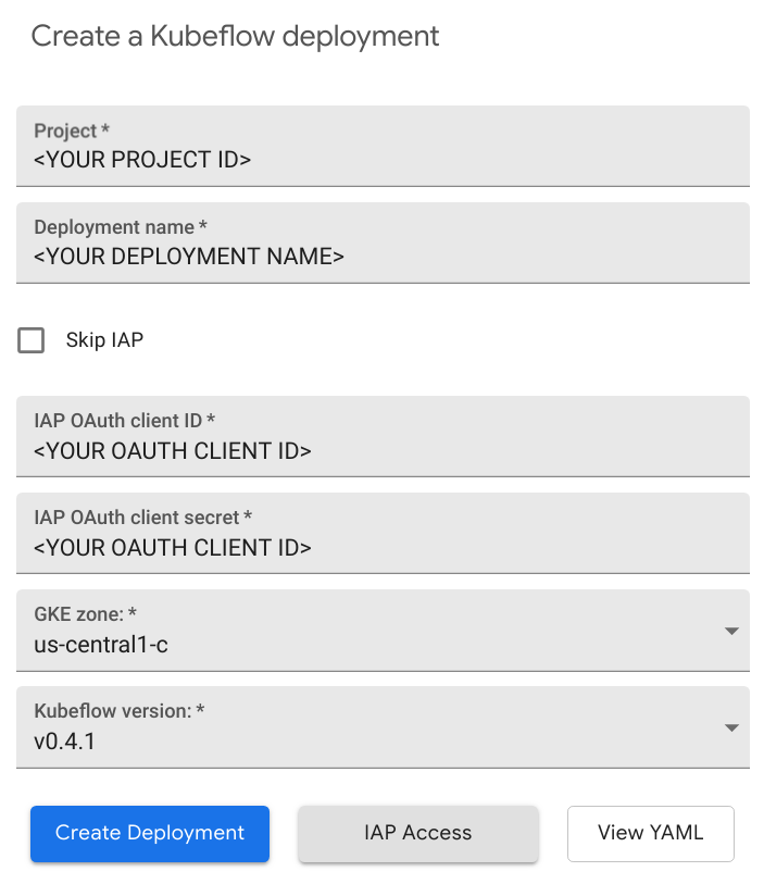
<deployment_name>as you used when setting up theDEPLOYMENT_NAMEenvironment variable earlier in this tutorial. - The following screenshot shows the Kubeflow deployment UI with hints about the value for each input field:
(Optional) If you want to examine your cluster while waiting for the Kubeflow dashboard to be available, you can use
kubectlto connect to your cluster:Connect your Cloud Shell session to the cluster:
gcloud container clusters get-credentials \
  ${DEPLOYMENT_NAME} --zone ${ZONE} --project ${PROJECT}
Switch to the
kubeflownamespace to see the resources on the Kubeflow cluster:kubectl config set-context $(kubectl config current-context) --namespace=kubeflowCheck the resources deployed in the
kubeflownamespace:kubectl get all
Access the Kubeflow UI, which becomes available at the following URI after several minutes:
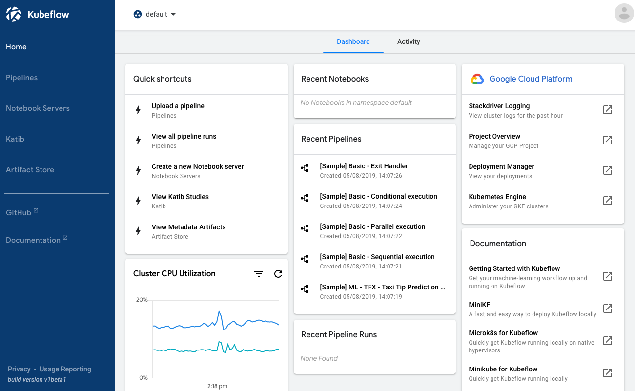
https://<deployment-name>.endpoints.<project>.cloud.goog/The following screenshot shows the Kubeflow UI:
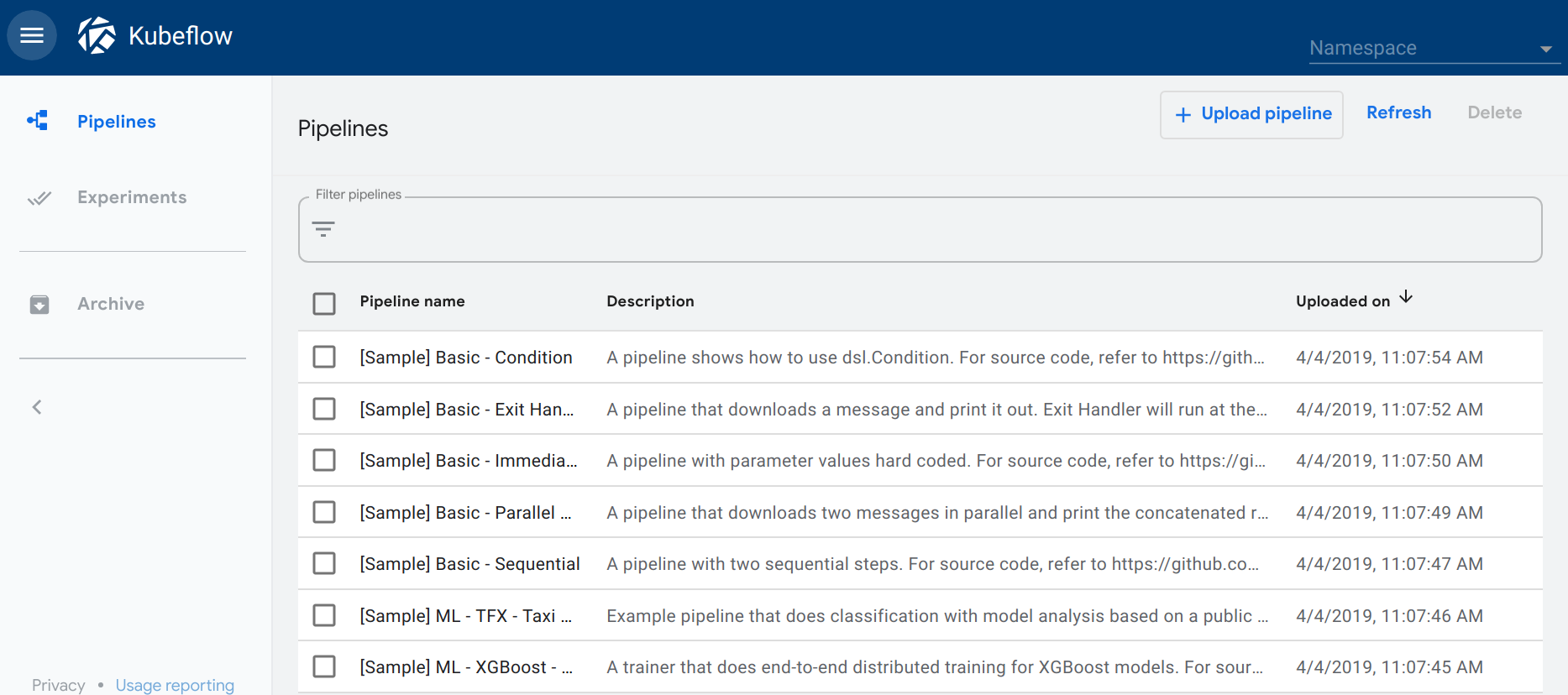
Click Pipelines to access the pipelines UI. The pipelines UI looks like this:
Notes:
While the deployment is running, you can watch your resources appear on the GCP console:
It can take 10-15 minutes for the URI to become available. Kubeflow needs to provision a signed SSL certificate and register a DNS name.
If you own/manage the domain or a subdomain with Cloud DNS then you can configure this process to be much faster. See kubeflow/kubeflow#731.
Create a Cloud Storage bucket
The next step is to create a Cloud Storage bucket to hold your trained model.
Cloud Storage is a scalable, fully-managed object/blob store. You can use it for a range of scenarios including serving website content, storing data for archival and disaster recovery, or distributing large data objects to users via direct download. This tutorial uses Cloud Storage to hold the trained machine learning model and associated data.
Use the gsutil mb command to create a storage bucket. Your
bucket name must be unique across all of Cloud Storage.
The following commands create a bucket in the region that corresponds to the
zone which you specified earlier in the tutorial:
export BUCKET_NAME=${PROJECT}-${DEPLOYMENT_NAME}-bucket
export REGION=$(gcloud compute zones describe $ZONE --format="value(region.basename())")
gsutil mb -c regional -l ${REGION} gs://${BUCKET_NAME}
Prepare your pipeline
To simplify this tutorial, you can use a set of prepared files that include the pipeline definition and supporting files. The project files are in the Kubeflow examples repository on GitHub.
Download the project files
Clone the project files and go to the directory containing the MNIST pipeline example:
cd ${HOME}
git clone https://github.com/kubeflow/examples.git
cd examples/pipelines/mnist-pipelines
As an alternative to cloning, you can download the Kubeflow examples repository zip file.
Set up Python
You need Python 3.5 or above. This tutorial uses Python 3.7. If you don’t have a Python 3 environment set up, install Miniconda as described below:
In a Debian/Ubuntu/Cloud shell environment, run the following commands:
apt-get update
wget https://repo.continuum.io/miniconda/Miniconda3-latest-Linux-x86_64.sh
bash Miniconda3-latest-Linux-x86_64.sh
In a Windows environment, download the installer and make sure you select the “Add Miniconda to my PATH environment variable” option during the installation.
In a Mac environment, download the installer and run the following command:
bash Miniconda3-latest-MacOSX-x86_64.sh
Create a clean Python 3 environment (this tutorial uses Python 3.7):
conda create --name mlpipeline python=3.7
conda activate mlpipeline
If the conda command is not found, be sure to add Miniconda to your path:
export PATH=MINICONDA_PATH/bin:$PATHInstall the Kubeflow Pipelines SDK
Install the Kubeflow Pipelines SDK, along with other Python dependencies defined
in the requirements.txt file:
pip install -r requirements.txt --upgradeCompile the sample pipeline
The pipeline is defined in the Python file mnist_pipeline.py which you
downloaded from GitHub. When you execute that Python file, it compiles the
pipeline to an intermediate representation which you can then upload to the
Kubeflow Pipelines service.
Run the following command to compile the pipeline:
python3 mnist_pipeline.pyAlongside your mnist_pipeline.py file, you should now have a file called
mnist_pipeline.py.tar.gz which contains the compiled pipeline.
Run the pipeline
Go back to the the Kubeflow Pipelines UI, which you accessed in an earlier step of this tutorial. Now you’re ready to upload and run your pipeline using that UI.
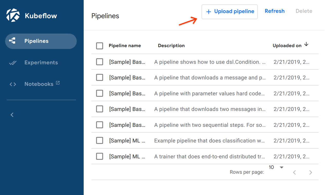
Click Upload pipeline on the Kubeflow Pipelines UI:
Upload your
mnist_pipeline.py.tar.gzfile and give the pipeline a name: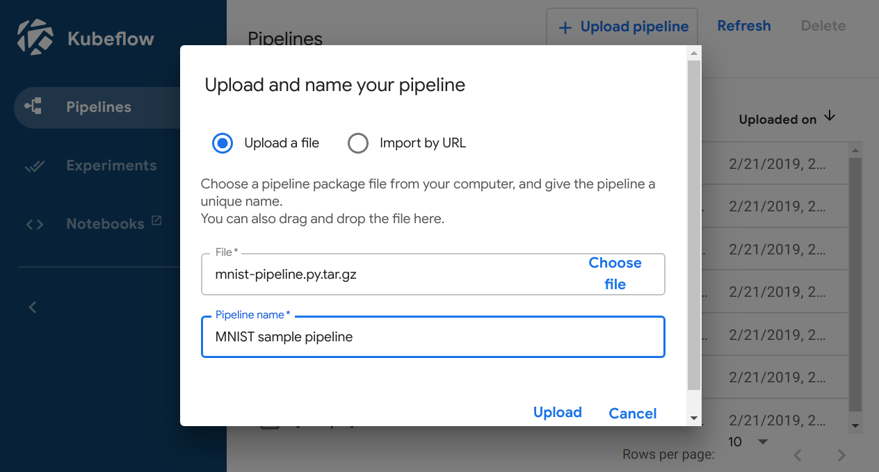
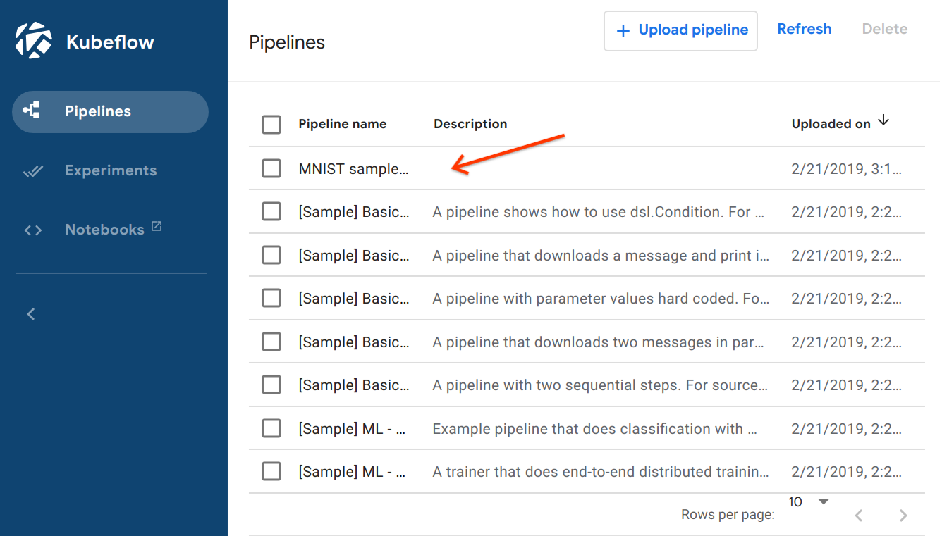
Your pipeline now appears in the list of pipelines on the UI. Click your pipeline name:
The UI shows your pipeline’s graph and various options. Click Create run:
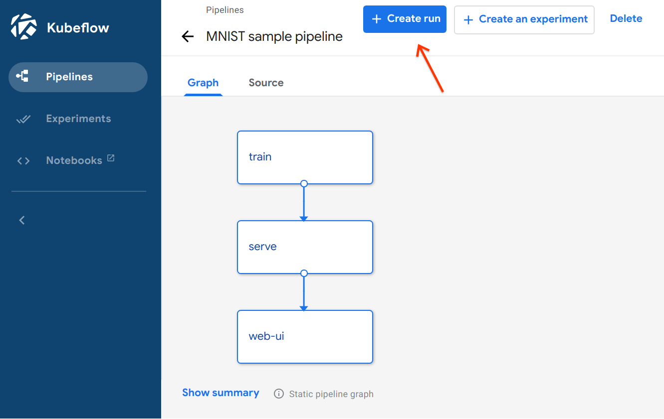
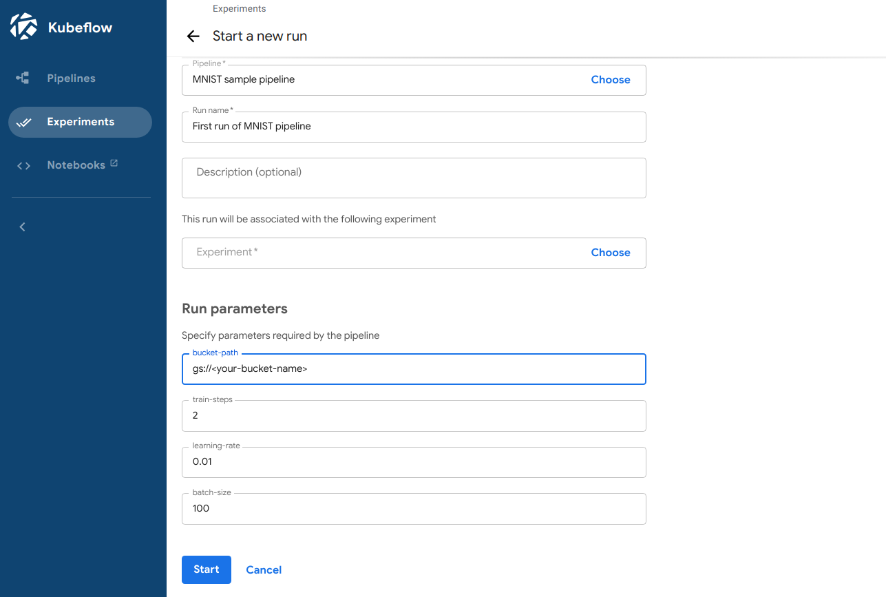
Supply the following run parameters:
- Run name: A descriptive name for this run of the pipeline. You can submit multiple runs of the same pipeline.
- bucket-path: The Cloud Storage bucket that you created earlier to hold the results of the pipeline run.
The sample supplies the values for the other parameters:
- train-steps: The number of training steps to run.
- learning-rate: The learning rate for model training.
- batch-size: The batch size for model training.
Then click Start:
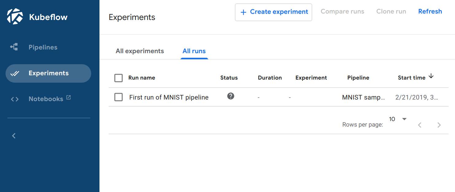
The pipeline run now appears in the list of runs:
Click the run to see its details. In the following screenshot, the first two components (
trainandserve) have finished successfully and the third component (web-ui) is still running: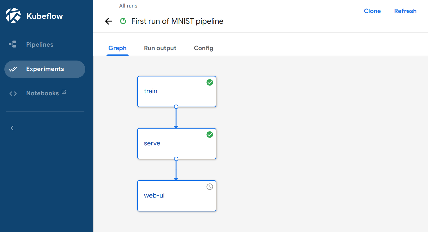
Click on any component to see its logs.
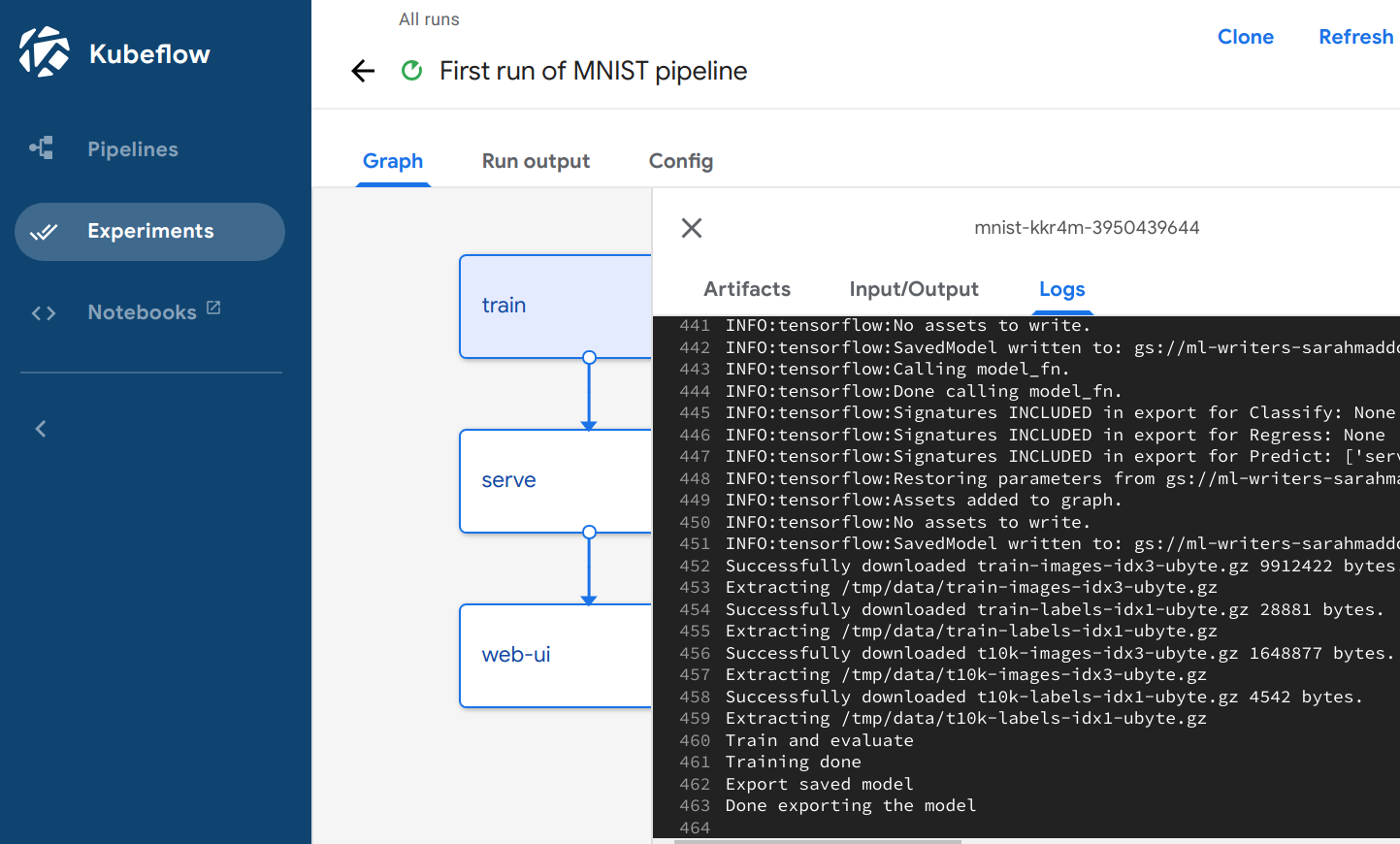
When the pipeline run is complete, look at the logs for the
web-uicomponent to find the IP address created for the MNIST web interface. Copy the IP address and paste it into your web browser’s address bar. The web UI should appear.Below the connect screen, you should see a prediction UI for your MNIST model.

Each time you refresh the page, it loads a random image from the MNIST test dataset and performs a prediction. In the above screenshot, the image shows a hand-written 7. The table below the image shows a bar graph for each classification label from 0 to 9. Each bar represents the probability that the image matches the respective label.
Notes:
- You can find your trained model data in the bucket path you entered in step 5 of this procedure.
Understanding the pipeline definition code
The pipeline is defined in the Python file mnist_pipeline.py which you
downloaded from GitHub. The following sections give an overview of the content
of that file.
Decorator
The @dsl.pipeline decorator provides metadata about the pipeline:
@dsl.pipeline(
  name='MNIST',
  description='A pipeline to train and serve the MNIST example.'
)
Function header
The mnist_pipeline function defines the pipeline. The function includes a
number of arguments which are exposed in the Kubeflow Pipelines UI when you
create a new run of the pipeline.
Although you pass these arguments as strings, the arguments are of type
kfp.dsl.PipelineParam.
def mnist_pipeline(model_export_dir='gs://your-bucket/export',
                   train_steps='200',
                   learning_rate='0.01',
                   batch_size='100'):
The training component (train)
The following block defines the train component, which handles the training
of the ML model:
train = dsl.ContainerOp(
    name='train',
    image='gcr.io/kubeflow-examples/mnist/model:v20190304-v0.2-176-g15d997b',
    arguments=[
        "/opt/model.py",
        "--tf-export-dir", model_export_dir,
        "--tf-train-steps", train_steps,
        "--tf-batch-size", batch_size,
        "--tf-learning-rate", learning_rate
        ]
).apply(gcp.use_gcp_secret('user-gcp-sa'))
A component consists of a
kfp.dsl.ContainerOp
object with a name and a container path. The container image for
the MNIST training component is defined in the MNIST example’s
Dockerfile.model.
The training component runs with access to your user-gcp-sa secret, which
ensures the component has read/write access to your Cloud Storage bucket for
storing the output from the model training.
The model serving component (serve)
The following block defines the serve component, which serves the trained
model for prediction:
serve = dsl.ContainerOp(
    name='serve',
    image='gcr.io/ml-pipeline/ml-pipeline-kubeflow-deployer:\
            7775692adf28d6f79098e76e839986c9ee55dd61',
    arguments=[
        '--model-export-path', model_export_dir,
        '--server-name', "mnist-service"
    ]
).apply(gcp.use_gcp_secret('user-gcp-sa'))
serve.after(train)
The serve component differs from the train component with respect to
how long the service lasts. While train runs a single container and then
exits, serve runs a container that launches long-lived resources in the
cluster.
The ContainerOP takes two arguments:
- A path pointing to the location of your trained model.
- A server name.
The component creates a Kubeflow
tf-serving
service within the cluster. This service lives on after the pipeline has
finished running.
You can see the Dockerfile used to build this container in the
Kubeflow Pipelines repository.
Like the train component, serve requires access to the user-gcp-sa secret
for access to the kubectl command within the container.
The serve.after(train) line specifies that this component must run
sequentially after the train component is complete.
The web UI component (web-ui)
The following block defines the web-ui component, which displays a simple
web page. The web application sends an image (picture) to the trained model and
displays the prediction results:
web_ui = dsl.ContainerOp(
    name='web-ui',
    image='gcr.io/kubeflow-examples/mnist/deploy-service:latest',
    arguments=[
        '--image', 'gcr.io/kubeflow-examples/mnist/web-ui:\
                v20190304-v0.2-176-g15d997b-pipelines',
        '--name', 'web-ui',
        '--container-port', '5000',
        '--service-port', '80',
        '--service-type', "LoadBalancer"
    ]
).apply(gcp.use_gcp_secret('user-gcp-sa'))
web_ui.after(serve)
Like serve, the web-ui component launches a service that continues to exist
after the pipeline is complete. Instead of launching a Kubeflow resource, the
web-ui component launches a standard Kubernetes deployment/service pair. You
can see the Dockerfile that builds the deployment image in the
./deploy-service/Dockerfile
that you downloaded with the sample files. This image runs the
gcr.io/kubeflow-examples/mnist/web-ui:v20190304-v0.2-176-g15d997b-pipelines
container, which was built from the MNIST example’s
web-ui Dockerfile.
This component provisions a LoadBalancer service that gives external access to a
web-ui deployment launched in the cluster.
The main function
The main function compiles the pipeline, converting the Python program to
the intermediate YAML representation required by the Kubeflow Pipelines service
and zipping the result into a tar.gz file:
if __name__ == '__main__':
  import kfp.compiler as compiler
  compiler.Compiler().compile(mnist_pipeline, __file__ + '.tar.gz')
Clean up your GCP environment
Run the following command to delete your deployment and related resources:
gcloud deployment-manager --project=${PROJECT} deployments delete ${DEPLOYMENT_NAME}
Delete your Cloud Storage bucket when you’ve finished with it:
gsutil rm -r gs://${BUCKET_NAME}
As an alternative to the command line, you can delete the various resources using the GCP Console.
Next steps
Build your own machine-learning pipelines with the Kubeflow Pipelines SDK.
Feedback
Was this page helpful?
Glad to hear it! Please tell us how we can improve.
Sorry to hear that. Please tell us how we can improve.